The magnetic field experiment IMSC

IMSC is composed of 3 orthogonal magnetic antennae (search coil type) linked to a pre-amplifier unit with a shielded cable of 80cm. (see Figure 1). The search coil magnetometer consists of a core in permalloy (high permeability material) on which are wound a main coil with several thousand turns (12000) of copper wire and a secondary coil with a few turns. The core is a 170 mm rod with a 4 x 4 mm cross-section. The induced voltage in the main coil is where µ_reff is the relative effective permeability, N the number of wire turns, S the cross section of the core, B the magnetic induction outside the core, aligned with the core. The coefficient µ_reff strongly depends on the ratio between the length and the diameter of the core, and on the permeability of the core. The secondary coil is used as a flux feedback, to create a flat frequency response on a bandwidth centred on the resonance frequency of the main coil. An electrostatic screen (comb shaped flexible printed circuit) connected to the signal ground maintains a uniform potential around the windings. The rod, the windings, the electrostatic screen, and the output cable are potted inside an epoxy tube (180 mm long, external diameter 20 mm).The three antennas are assembled in a nut like structure optimised for minimum weight (430 g with a cable of 80 cm). The unity is mounted at the end of a 1.9 m boom in order to decrease the intensities of the interferences coming from the satellite (see Figure 2). The pre-amplifier is located at 80 cm on the same boom. Its role is to amplify the 3 signals before filtering and analog-digital conversion. It contains a temperature sensor and its weight is 300 g.

In the VLF range, the flat frequency response of the frequency band is going from 100 Hz up to 17.4 kHz. These are the cut-off frequencies at 3dB, the slopes of the filter being +6 dB/octave and -12 dB/octave, respectively.

In order to check the good operation of the antennas, a calibration sequence can be implemented when the experiment is switched on and then every 4, 8 or 12 minutes (fixed by telecommand). During this sequence a sum of two sinusoids at 625 Hz and 10 kHz is sent during one second in burst mode and four seconds in survey mode.

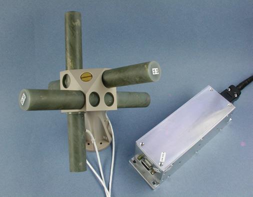
Figure 1: The magnetic search-coil IMSC and its pre-amplifier.

The strategy to record the data

There are two main modes of operation: a burst mode which is triggered when the satellite is above given seismic zones (see Figure 4), and elsewhere a survey mode. The corresponding recorded data are

• in the BURST MODE

– waveforms of the three magnetic components in the ELF range up to 1 kHz,

– waveforms of one magnetic component (selected among the three by telecommand) in the VLF range up to 17 kHz,

• in the SURVEY MODE

– spectra of one magnetic component (selected among the three by telecommand) up to 17 kHz. Three possible combinations of frequency and time resolutions can be selected by telecommand (see table 1).

Type	Samples ( FFT input)	Average spectra	Time resolution	Average frequencies	Frequency resolution	Points of spectrum	TM flow
0	2048	40	2.048 s	1	19.53 Hz	1024	4 kb/s
1	2048	10	0.512 s	1	19.53 Hz	1024	16 kb/s
2	2048	40	2.048 s	4	78.125 Hz	256	1 kb/s

Table 1. VLF spectrogram characteristics in Survey mode.

It must be noted that during the burst mode and for simplification of the data processing, a VLF spectrum similar to the one which is calculated in survey mode can be implemented. Before the FFT, a Blackman-Harris window is applied on the samples.

In addition, whatever is the mode, either a magnetic or an electric component in the VLF range is used as input for the onboard neural network .

The ELF and VLF waveforms are sent in telemetry with 2 bytes resolution.

The averaged spectrum values G_v(k) onboard the scientific payload computer are with four bytes and to reduce this dynamic in the telemetry, a logarithmic compression on one byte is done in order to have a power with 256 levels which can be directly transform in an image with 256 colors. Then all frequency components of the VLF spectrum (256 or 1024) G_TM(k) given by

where Round(x) gives the nearest integer to x, are sent in telemetry as bytes together with the two gains (a minimum G_min and a maximum value G_max which can be modified by telecommand) which are used to increase the dynamic. Then the classical transfer function is applied to obtain physical values.

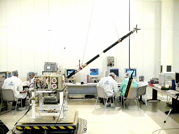
Figure 2: IMSC mounted at the end of its boom during integration tests.

Figure 3: Sensitivity of the search-coil antenna as function of frequency. The black curve is related to the theory and the red curve includes the complete chain of analysis.

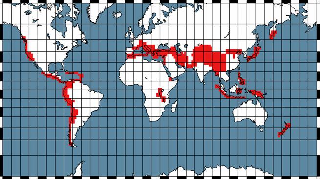
Figure 4: The zones where the experiment will be in burst are indicated in red.